Plot descriptive summary statistics of multiple variables

This function plots distributions (histograms/barplots) and shows basic summary statistics (e.g., median [Q1, Q3], % missing etc.) for multiple variables.

Usage

plot_summary(
  data,
  plot_vars = NULL,
  facet_group = NULL,
  show_stats = TRUE,
  prct = FALSE,
  base_size = NULL,
  color = "lightblue",
  ...
)

Arguments

data: (data.frame | data.table)
Table containing data to be plotted.
plot_vars: (character | list)
Character vector or list of variables to be plotted. If no plot_vars input is provided, the function will automatically plot all variables, ignoring any encounter/patient/physician IDs and date-time variables.
facet_group: (character)
Name of variable to be used as facet variable. This only works if plot_vars only specifies 1 variable to be plotted. Users can then create separate subplots per facet_group level, for example, to plot separate histograms/ barplots for each hospital (facet_group = "hospital_num")/
show_stats: (logical)
Flag indicating whether to show descriptive stats above each plot.
prct: (logical)
Flag indicating whether y-axis labels should show percentage (%). If FALSE (default), counts (n) will be shown.
base_size: (numeric)
Numeric input defining the base font size (in pts) for each subplot. By default, the function will automatically determine an appropriate size depending on the number of subplots (base_size = 11 if a single subplot).
color: (character)
Plotting color used for "fill". Default is R's built-in "lightblue".
...: Additional arguments passed to ggpubr::ggarrange() that allow for finer control of subplot arrangement (e.g., ncol, nrow, widths, heights, align etc.; see ? ggarrange for more details).

Value

(ggplot)
A ggplot figure with subplots showing histograms/ barplots for all variables specified in plot_vars.

Note

These plots are not meant as publication-ready figures. Instead, the goal of this function is to provide a quick and easy means to visually inspect the data and obtain information about distributional properties of a wide range of variables, requiring just a single line of code.

Additional inputs when providing `plot_vars` as a list

When plot_vars are provided as a list, users can specify additional characteristics for each individual variable, such as:

class (character): variable type, e.g., "numeric", "character", "logical" etc.
sort (character): for categorical variables, whether to sort bars in ascending ("^a") or descending (starting with "^d") frequency
binwidth/bins/breaks: for numeric/integer variables, specifying the histogram bins
normal: for numeric/integer variables, whether to assume normal distribution (will show mean [SD] if show_stats = TRUE)

Examples

# simulate GEMINI data table
admdad <- dummy_ipadmdad(
  n = 10000,
  n_hospitals = 20,
  time_period = c(2015, 2022)
)

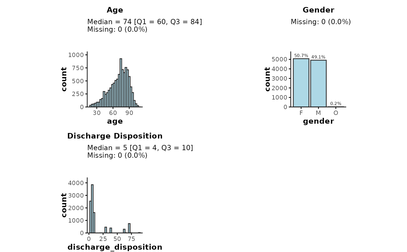
## Providing plot_vars as a character vector
plot_summary(
  data = admdad,
  plot_vars = c("age", "gender", "discharge_disposition")
)
#> `stat_bin()` using `bins = 30`. Pick better value with `binwidth`.
#> `stat_bin()` using `bins = 30`. Pick better value with `binwidth`.
#> `stat_bin()` using `bins = 30`. Pick better value with `binwidth`.
#> `stat_bin()` using `bins = 30`. Pick better value with `binwidth`.


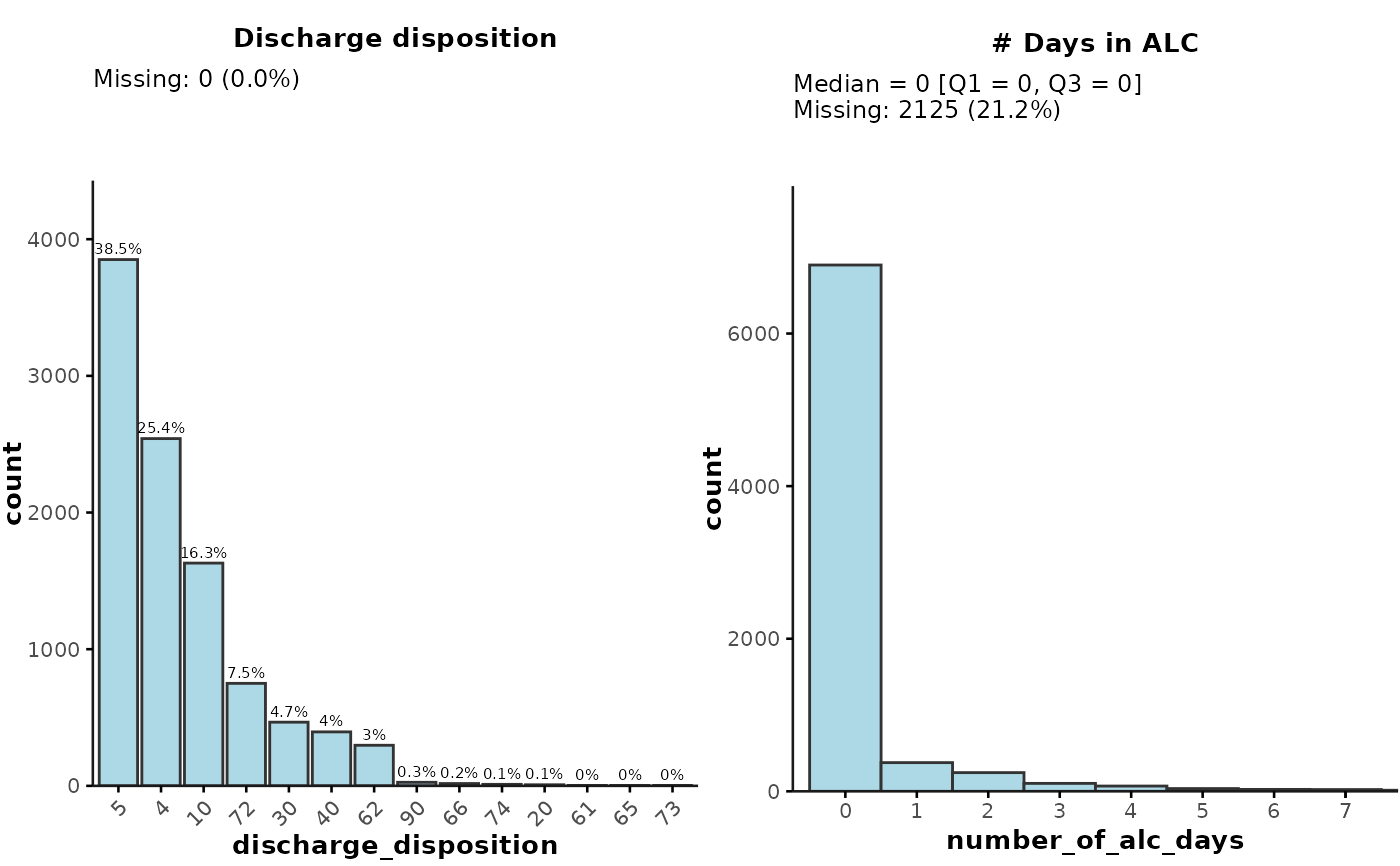
## Providing plot_vars as a list input
plot_summary(
  admdad,
  plot_vars = list(
    `Discharge disposition` = list(
        plot_var = "discharge_disposition",
        class = "character",
        sort = "desc"
    ),
    `# Days in ALC` = list(
        plot_var = "number_of_alc_days",
        binwidth = 1,
        breaks = seq(0, 7, 1)
    )
  )
)